Goals
My goal here is not to provide a detailed how-to for creating a machine learning system. Most people who do anything with machine learning will be using systems already built into tools such as Splunk, Elastic Search or other such software. I’m only seeking to provide some basic understanding of how machine learning systems work.
An analogy would be that you don’t need to understand how a differential gear system works in detail, but a basic knowledge of what it is doing is useful to understand when you should lock the differential on an off-road vehicle.
Similarity as Determined by Human Intelligence
Consider that you have a set of documents, be they a collection of news articles, encyclopedia entries, essays, customer comments, etc. You as a human are tasked with identifying which documents are similar. What does similarity mean?
A human can read the documents and develop an understanding of them. He can form a mental ontology to classify them into categories. If they are news articles, this one is about politics. This one about the economy. This one argues against Marxism. This one against Capitalism.
Ontology: A set of concepts and categories in a subject area or domain that shows their properties and the relations between them.
OED
Although so-called Deep Learning attempts to mimic a hypothetical model of human learning, it is still not real human intelligence and is computationally demanding. Instead, we usually take shortcuts that will be more practical, if not as powerful.
Big Bag of Words
Specific concepts have unique vocabularies
Assumption 1
Our first simplification is to throw out all knowledge of grammar and even word meanings. We treat documents as a “big bag of words” without any grammatical relationship between them, and rely on presence or absence of individual words to measure the similarity of documents.
Words have Weight
Some words have more importance in measuring the ontological similarity of documents. To estimate this importance, we make some assumptions about the relationship between words and concepts.
Term Frequency
Specific concepts use certain words with greater frequency.
Assumption 2
We incorporate Assumption 2 by weighting each word by the number of times it occurs in each document. This weight is referred to as the Term Fequency (TF).
Inverse Document Frequency
Specific concepts use certain words that are less likely
Assumption 3
to be used by other concepts.
We incorporate Assumption 3 by weighting each word by the reciprocal of the portion of documents it occurs in. A word that occurs in every document gets weight 1. One that occurs in only 1% of the documents gets weight 100. This factor is referred to as the Inverse Document Frequency (IDF). We are essentially assuming that documents that share a rare word are more likely to be similar.
The two factors are combined by multiplying them. This combined weighting factor is referred to by the acronym TF-IDF.
Stop Words
Some words intrinsically carry less semantic information
Assumption 4
and so are less indicative of concepts
regardless of their TF-IDF weight.
Words like the, a, preprositions, helping verbs, and the like carry little specific semantic information on their own related to ontological concepts. They are all very common, having a high term frequency, but a low inverse document frequency. These words, referred to as stop words, are left out of the calculation, effectively giving them a weight of zero. Most turn-key systems will have a list of stop words built into them.
Stemming
For our purposes, it generally doesn’t matter if a verb is past or future tense. We’ve already omitted helping verbs as stop words above. We might as well discard inflections and conjugations as well, reducing words to their root forms.
There are several heuristic algorithms available in most natural language processing packages for chopping off the prefixes and suffixes added to words. This is referred two as stemming. The better algorithms also include dictionaries for stemming irregular forms as well. Thus go, gone, went, goes, and going will all be stemmed to go.
Vectors
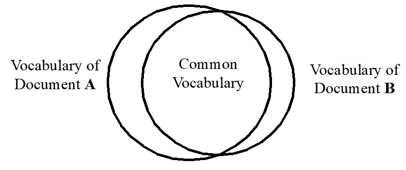
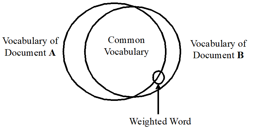
We could continue using the Venn diagram like in Figure 1 above. A key difference with that previous diagram is that because TF-IDF is being utilized and different documents have different term frequencies, some of a word’s weight will be in the Common Vocabulary section, and some will be in a specific document’s unique vocabulary section.
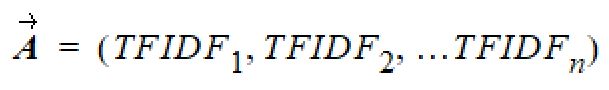
However, there is an alternative approach used that can be concisely expressed as mathematical formulas with calculations done with readily available math packages. This approach is to express each document as an n-dimensional vector of weighted terms.
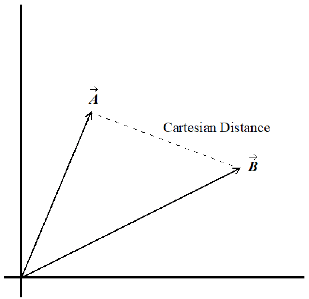
Similar documents will be closer together in this n-dimensional Euclidean space, and dissimilar documents will be further apart. This is difficult for us to imagine, living in an only 3-dimensional world. However, we can easily illustrate the similarity of two documents in two dimensions. Two vectors are defined by three points: the point of origin and the end points of the two vectors. Two points define a 1-dimensional line, even when the points are located in n-dimensional space. The third point defines a 2-dimensional plane within that space. It is always possible to rotate our perspective around to look at the 2-dimensional plane within the n-dimensional space that contains our two vectors.
Size Doesn’t Matter
Imagine that you have a largish document about a specific concept. Now imagine that you edit a copy of that document to condense it, removing redundancies and writing shorter sentences, being in general more concise. The new document still discusses the same concept and makes all the same points about that concept. It still uses the same vocabulary for the most part. It probably even uses the words in the same proportions. But the length of the document and the term frequency of its words are reduced proportionally (or nearly so).
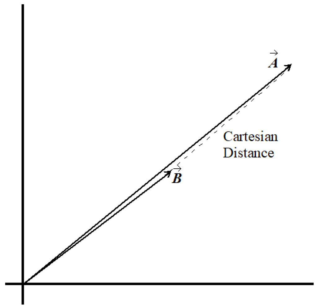
The Cartesian distance between these two documents in Figure 4 is nearly the same as in Figure 3, even though they are ontologically almost identical. The length of the treatments of a concept really doesn’t matter much to us for the purpose of measuring their similarity.
For this reason, we normalize the documents’ vectors to have a length of one unit.
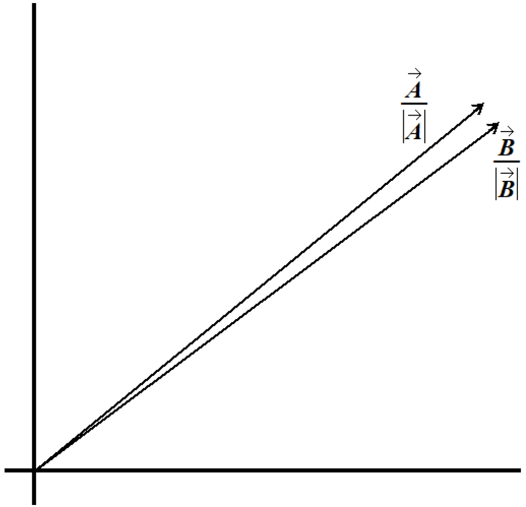
Cosine Similarity
Because the TF-IDF values are never negative, the vectors for two documents will always be within 90 degrees of each other. Consider the two-dimensional case; the two vectors will be in the upper right quadrant. Add a third dimension. No matter how large the third coordinate, the vectors can only approach asymptotically the third dimension, which being perpendicular, limits them to becoming no more than 90 degrees apart. The only way they can exceed 90 degrees, is if one takes on a negative coordinate while the other takes on a positive one. For n dimensions, we can always rotate our perspective to two dimensions, so inductively we can see that for any number of dimensions, they’ll be within 90 degrees.
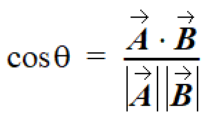
This gives the Cartesian distance a range of 0.0 (for maximum similarity) to the square root of 2.0 (for maximum dissimilarity).
A range of 0.0 (for maximum dissimilarity) to 1.0 (for maximum similarity) would be more intuitive. As it happens there is a simple way to get that: The cosine of the angle between the vectors. Better, there is a simple formula for calculating that cosine. This calculation is referred to as cosine similarity.
Continued in Part 2…
Part two will examine some uses of TF-IDF and Cosine Similarity…
