Category: Software Development

Spreadsheets Are Programming Too

Watching the stock market recover dramatically since the bottom was hit in 2009 when all hopes for not dying at my desk in a windowless office somewhere were dashed, I’m suddenly in a mind to work out how best to budget retirement though it’s still likely ten years or more away. A popular method is called bucket budgeting, where retirement savings are divided into three (or more) buckets with increasing amounts of risk (and returns) for the near, medium, and far term.

I decided to program a spreadsheet to simulate decades of retirement under different assumptions, using various stochastic models for future market behavior as well as replaying historic returns for various periods. This spreadsheet may be downloaded below for your own adaptation and experiments.

Disclaimers: Past history is not indicative of future performance. I am not a financial advisor. I do not warrant this spreadsheet to be free of defects in any way. This blog is not financial advice, but rather programming advice on how one might program a simulation. You should make your own assumptions and models and draw your own conclusions in concert with a professional fiduciary financial advisor. The assumptions and tradeoffs I make for myself are probably not the same ones you should make.

An Illustrated Tour of the Spreadsheet

Parameters

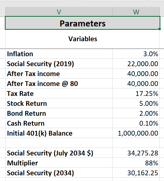
This block of values defines various parameters you can set to tune the simulation.

Inflation. This sets what inflation is expected to be. It has been running below 2% for a few years now, but something like 3% or even 4% is more normal.

Social Security (2019). This is the social security benefit per year in 2019 dollars, which is the value given by most social security calculators. By the way, none of the financial numbers here are my actual numbers. They are contrived for illustration purposes only.

After Tax Income. Working from my budget for today, I remove those items like mortgage that I won’t be paying in retirement, and add those I have that I don’t have now but hope to in retirement, like hobbies or travel, to come up with a realistic desired post-retirement income level.

After Tax Income @ 80. A different income level can be set for old age. It might be lower because one travels less, or more to pay for a nursing home.

Tax Rate. This is an estimate of federal, state, and local income taxes. It will vary depending on jurisdiction as well as on the size of the social security benefit. I expect an approximation in the right neighborhood is good enough. But politics might require radical revisions to this estimate in the future.

Stock Return. This estimates the amount stocks will grow per year. The long term average since 1901 is a little over 5%, but around 7% since WW II, about 9% since Reagonomics, and even higher since the Great Recession. The “Rule of 25”, also called the “4% Rule”, is basically based on 5% growth since it looks at all 30 year periods since 1901.

The spreadsheet also allows setting returns for individual years (the Stock Variation column). In that case, this number is added to the Stock Variation value for a given year. This permits simulating an index fund that beats or falls short of the actual market numbers.

Bond Return. This estimates the return on bonds in the middle bucket of this simulation.

Cash Return. This estimates the return on the cash in the near-term bucket of this simulation. It should probably be something near zero these days.

Initial 401(k) Balance. This is the 401(k) balance on the day of retirement.

Social Security (July 2034 $). This is an inflation adjusted estimate of the social security benefit for the year one begins collecting social security. It is calculated from the above parameters. For me, this is 15 years in the future. You will need to change this for your own age and planned date for collecting social security. I’m assuming I’ll delay until age 70 while retiring at 65.

Multiplier. Unfortunately, social security will go bankrupt the same year I start collecting it. At that time, it will only be able to pay out what it also collects that year, which is 77 cents on the dollar of the defined benefit. I’m guessing a combination of tax increases and benefit cuts will eventually be enacted, so I split the difference and guess it will pay 88 cents on the dollar.

Social Security (2034). So this will be the actual estimated social security benefit for the year of retirement. All the social security numbers are for the full year rate and should be amortized in the spreadsheet for the portion of the year one is actually 70.

Time

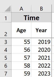
Age. This is the age one turns each year. First row sets the intial age, then subsequent rows add one to the previous row. Depending on personal preference, one might want to have it be one’s age at the beginning of the year. It’s purely a convenience value and not used for any calculations directly.

Year. This is the calendar year. It is calculated the same way as age, setting an initial value explicitly and adding one to the previous row on subsequent rows.

Income Goals

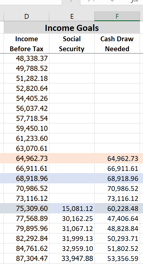
Income Before Tax. The first row is calculated from the parameters, dividing after tax income by one minus the tax rate. Subsequent years are inflation adjusted. There is an adjustment at age 80 for the difference in income that can be configured for age 80 and later in the Parameters. It simply scales the regular calculation proportionally.

Social Security. Since I’m born near the middle of the year, the first social security row half the Social Security (2034) in the Settings section. Subsequent years are full collection and inflation adjusted. This will need to be adjusted for individual situations.

There has been talk about changing the CPI index that social security is adjusted on, but I’m not modeling that possibility at this time.

Cash Draw Needed. This is the actual amount of cash drawn from the 401(k) each year of retirement. I’m assuming I’ll retire at the beginning of the year I turn 65. This could be adjusted for midyear retirement (by proportionally amortizing the calculated value) or for retiring a different year. The calculation is simply Income Before Tax minus Social Security.

Bucket Goals

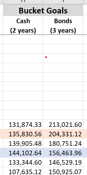
Deep dives in the stock market usually recover in about five years or less, so I somewhat arbitrarily chose five years worth of income as the horizon for the Cash and Bonds buckets. Others may or even should choose other time horizons.

Cash. The cash bucket has the goal of having a balance of the next two years of 401(k) draw needed.

Bonds. The bonds bucket has the goal of having the following three years of 401(k) draw needed.

When the stock market is down, the plan is to defer transfers from stocks to bonds until it recovers, draining the cash and bonds buckets until then, and then catch them back up once the stock market recovers.

Buckets

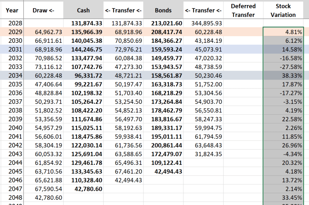
Now we come to the meat of the spreadsheet. This is where future history is simulated. For each row, money flows from right to left. Money is transferred at the beginning of the year and balances represent the end of the year balance after transfers and then growth have occurred.

Draw <-. This is the amount taken out of Cash and is normally the number from Income Goals, but it is limited by the Cash balance, which is calculated as the previous year’s Cash balance plus the amount transferred into cash this year.

Cash. This is the amount of cash at the end of the year. It is previous year’s balance plus the transfer into cash minus the draw, then that summation multiplied by one plus the Cash Return rate from Parameters.

<- Transfer <-. Cash is replenished by transferring money from Bonds to Cash. The transfer is calculated as the amount of money needed to bring the Cash balance back up to this year’s goal after the draw is taken. It is limited by the amount of money in Bonds after funds have been transferred from Stocks to Bonds.

Bonds. This is the amount of money in Bonds at the end of the year. It is the previous year’s blance plus the transfer from Stocks minus the draw, then that summation multipled by one plus the Bonds Return rate from Parameters.

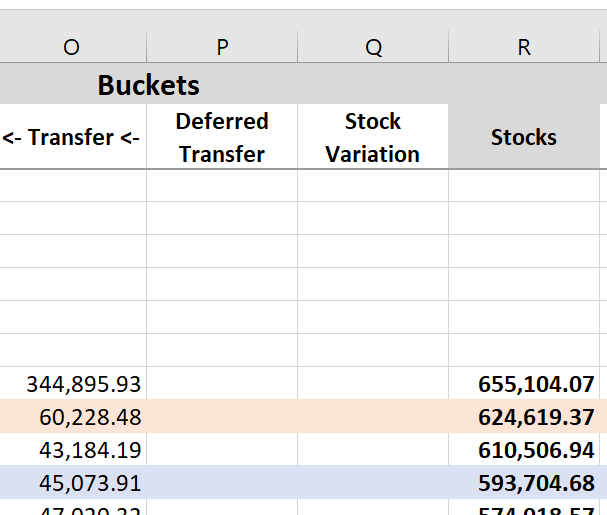
<- Transfer <-. Bonds are replenished by transferring money from Stocks to Bonds, unless they aren’t (more on this below). The transfer is calculated as the amount of money needed to bring the Bonds balance back up to this year’s goal after the transfer to Cash is done. It is limited by the amount of money in Stocks. It can also be adjusted by the Deferred Transfer, which see.

Deferred Transfer. If the market is down for some year, it might be desirable to not pull money from Stock until the market recovers, else losses are locked in. The amount to defer may be entered in this column. Bonds, and then Cash, will be drawn down instead then. The following year will catch up and re-fund Bonds unless it has a deferral too. When copying values from other cells into this column, be sure to paste as values.

Stock Variation. This will be discussed in detail in the following Stochastic Data section below and in the description of the Stocks column immediately below.

Stocks. The is the stock balance at the end of the year. After the transfer is made to Bonds, the balance is multipled by one plus the sum of Stock Return in Parameters and that year’s Stock Variation. So for a constant year-over-year growth, leave Stock Variation blank (zero). Variations relative to the Stock Return may be entered in the Stock Variation column. Or year-by-year returns may be specified by setting Stock Return to zero in Parameters and entering the actual return in Stock Variation rows. This is discussed in more detail below under Stochastic Data.

Stochastic Data

In the real world, the market does not go up year after year by a constant amount. These columns provide some data to paste into the Stock Variation column to stochastically model realistic variation. The equations of most of them include random numbers that get reëvaluated every time a cell gets updated. To do experiments with this data, be sure to use Excel’s Paste-as-Values feature to lock in a snapshot of the random values.

Random Variation. This provides normally distributed percentages. In Parameters give the average yearly Stock Return. Then Paste-as-Values numbers from this column. To change the standard deviation you’ll need to edit the equation in the cells as I didn’t parameterize it.

But in truth, this data hasn’t proven to be realistic. It comes up with long sequences of growth or decline much more often than happens in the real world. I suppose this could be useful for an extreme stress test of any set of parameters one wishes to try.

Historic Variation. This allows replaying of historic market behavior in the simulated future. There’s no random number generator used, so it’s OK, even suggested, that you copy the cells or equations into the Stock Variation column. Don’t copy the top most number (1901 in the illustration). Rather edit that number to set the initial year of returns to use.

Set the Stock Return in Parameters to zero as that value will be added to every Stock Variation number. Or set it to some small percentage to simulate an index fund beating or missing the Dow’s capital return. I usually use 1% to simulate dividends adding to the capital return. This applies for using Random Year and Random Decade columns too.

Random Year. This picks a random year’s return in the range of 1945 to 2018 for each year. The character of the market and its volatility was very different prior to then. This tends to look much more like real markets, although it can have “too many” bad or good years in a row sometimes.

Random Decade. This picks random ten-year spans’ returns for each decade of retirement. This repeats historic patterns of boom and bust fairly well, like Historic Variation, but with some scrambling so you aren’t locked into a comparatively small sample of years. This is what I use most of the time.

Results

Assumptions

The Parameters are set to de-personalized values. They also violate the 4% rule. With these settings, draw is a little over 6% once social security kicks in at 70 and much higher prior to that. This makes catastrophic failure of savings occur more often than if the 4% rule were followed. This was intentional as the 4% rule results in catastrophe less than 5% of the time and that invoves too many experiments get worst case scenarios.

Fixed Rate Returns.

Return	Age	Last Year	Last Draw
11%	125+	2089+	N/A
9%	99	2063	$87,528.45
7%	91	2055	$20,690.10
5%	87	2051	$24,938.24

The market has been approaching 11% returns lately. But the long term average since 1901 has been about 5.3%. So let’s look at how long money lasts for various fixed rate returns between 5 and 11 percent. This was done in the Bucket Model tab, setting different values for Stock Return in Parameters and leaving the Deferred Transfer and Stock Variation columns blank.

Random Decades.

Age	Last Year	Last Draw
91	2055	$25.73
83	2047	$17,549.85
87	2051	$15,941.36
95	2059	$75,044.79
84	2048	$65,189.22
86	2050	$2,323.56
114	2078	$8,554.19
90	2054	$79,491.73
125+	2089+	N/A
96	2060	$80,889.02

Now let’s apply some random decades and assuming beating the market by 1% for dividends. Using the Random Decades tab (a copy of the Bucket Model tab), I’ll set Stock Return to 1% and paste in the equations from the Random Decades column and recalculate ten times to see the variation we get.

As you can see, the results can be dramatically variable. You flaunt the 4% rule at your peril.

Strategies for Extending Savings.

Now let’s take a typical bad year where we run out of money at 84 in 2048 after only 19 years of retirement. I’m still using the Random Decades tab with the values from the Random Decades column pasted in as values so that they don’t change every time the spreadsheet recalculates.

The other “Random Decades” tabs all reference the Stock Variation column in the Random Decades tab so we can experiment with different strategies in parallel without having to set the Stock Variation column in each tab.

Random Decades (Deferred). The first stategy is to defer transfers from Stocks when the market is down until it recovers. This drains Bonds and Cash. Once the Market recovers, we refund Bonds and Cash.

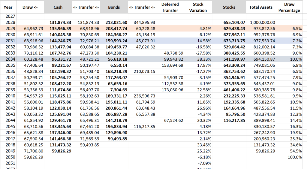
So, the market was down in 2032, so in 2033 no transfer from stock was made. This was signaled by copying a value from the Transfer column to the Deferred Transfer column.

I’ve not figured out a way to calculate deferrals automatically in the spreadsheet without programming some macros. Instead I just do a manual process.

Deferrals continue happening through 2035. After the growth in 2035, the market recovered and transfers were allowed to catch the other buckets up to plan again.

A similar situation occurs immediately afterwards. The net effect is that money holds out till late in 2050, a couple years longer than the base situation.

Random Decades (No Bonds). What if we dispensed with bonds altogether and just kept the cash bucket? We can’t defer quite as much because cash only has two years of buffer, so that third year we want to defer, we can only keep deferring the first two years of transfers, but little or no more.

For the sake of brevity (and laziness), I’ll not continue posting screenshots, and just summarize the results. The result for no bonds is running out of money in late 2054, a full four years later still.

Random Decades (No Cash). What if we also dispense with the cash bucket and just let it all sit in Stocks till we draw it down. No deferrals are done at all then. The result is running out of money in mid-2059, nearly five more years into the future!

Summary. It seems that almost always the losses one avoids from being able to draw from Cash or Bonds when the market is down are dwarfed by the gains one loses by holding cash and bonds for the duration of retirement.

I must reiterate, this is not financial advice. There are as many bucket strategies (and probably more) as there are advocates for bucket budgeting. One of them might do better. A better simulation of bonds returns similar to what I do for stocks might change the balance between avoiding loses and missing gains.

This blog entry is about how to program simulations with tunable assumptions. It illustrates techniques that can be expanded for a more complete simulation. The sample assumptions may be catastrophically poor. Your financial well being is your responsibility, not mine.

The following table summarizes when money runs out for the various strategies outlined above.

Strategy	Age	Last Year	Last Draw
All Three Buckets with No Deferrals	84	2048	$42,780.60
Deferral While Market Is Down	85	2049	$7,696.57
Deferral with No Bonds Bucket	86	2050	$71,291.21
No Bonds nor Cash Buckets	88	2052	$41,793.47

Stress Tests

So as a further experiment, what if one retired at the beginning of 2000, right at the start of the dot-com bust? In the simulation, I’ll copy the data for 2000 through 2018 and play those years on a loop so we get back-to-back-to-back-to-back major stock tankings. This historic data is conveniently off to the far right of the spreadsheet. The results are summarized in the following table.

Strategy	Age	Last Year	Last Draw
All Three Buckets with No Deferrals	82	2046	$24,798.56
Deferral While Market Is Down	86	2050	$58,826.29
Deferral with No Bonds Bucket	90	2047	$60,231.10
No Bonds nor Cash Buckets	93	2057	$16,914.71

Even with this extreme of a situation, it seems better to hold all stock by a wide margin.

Let’s go for even worse. Let’s loop 2000 through 2009. This would be a long term bear market for the entirety of retirement: a net loss every decade. Let’s further double the amount of initial savings to $2,000,000 so that the baseline retirement lasts an appreciable amount of time, till age 94.

Strategy	Age	Last Year	Last Draw
All Three Buckets with No Deferrals	94	2059	$78,138.33
Deferral While Market Is Down	97	2061	$31,775.66
Deferral with No Bonds Bucket	91	2059	$40,981.75
No Bonds nor Cash Buckets	90	2054	$54,283.43

Only in this most extreme situation does it appear the bucket scheme puts you ahead. But the down side here is considerably smaller than the upside during “normal” retirements.

I honestly didn’t expect this extreme of a difference. Spreadsheets can be notoriously difficult to get right. I’d rather be modeling this with something like MathLab, I think. But as I think about it, it seems right, with the market doubling every decade (or better of late) that five years of savings being held in cash and bonds could translate into much than that when held in stocks for 20 years or so.

What’s Next?

Given the possibility of extreme gains or loses during different periods of retirement, applying the 4% rule to pull out a constant amount (inflation adjusted) of money may not be the best approach. If the market turns into a real bear, it might be better to scale back the income a bit. If it turns into a raging bull, income might be increased significantly. I’m working on a model for dynamically adjusting income while stochastically modeling returns and still being assured (hopefully) of not running out of money too soon. Some day, I’ll turn it into a blog entry as well.